IC 1396A – The Elephant Trunk Nebula

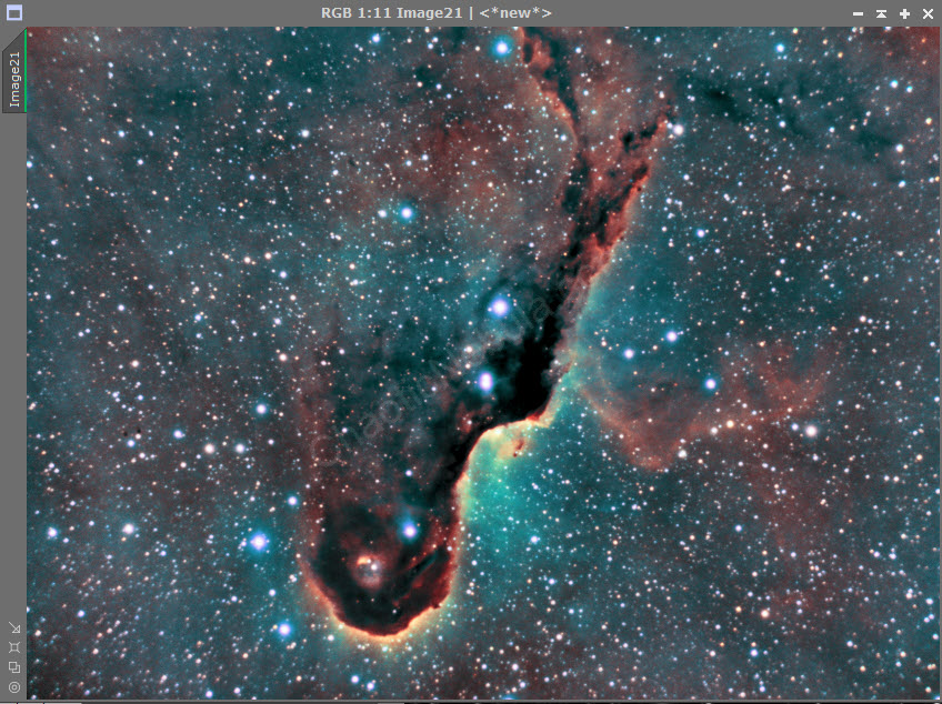
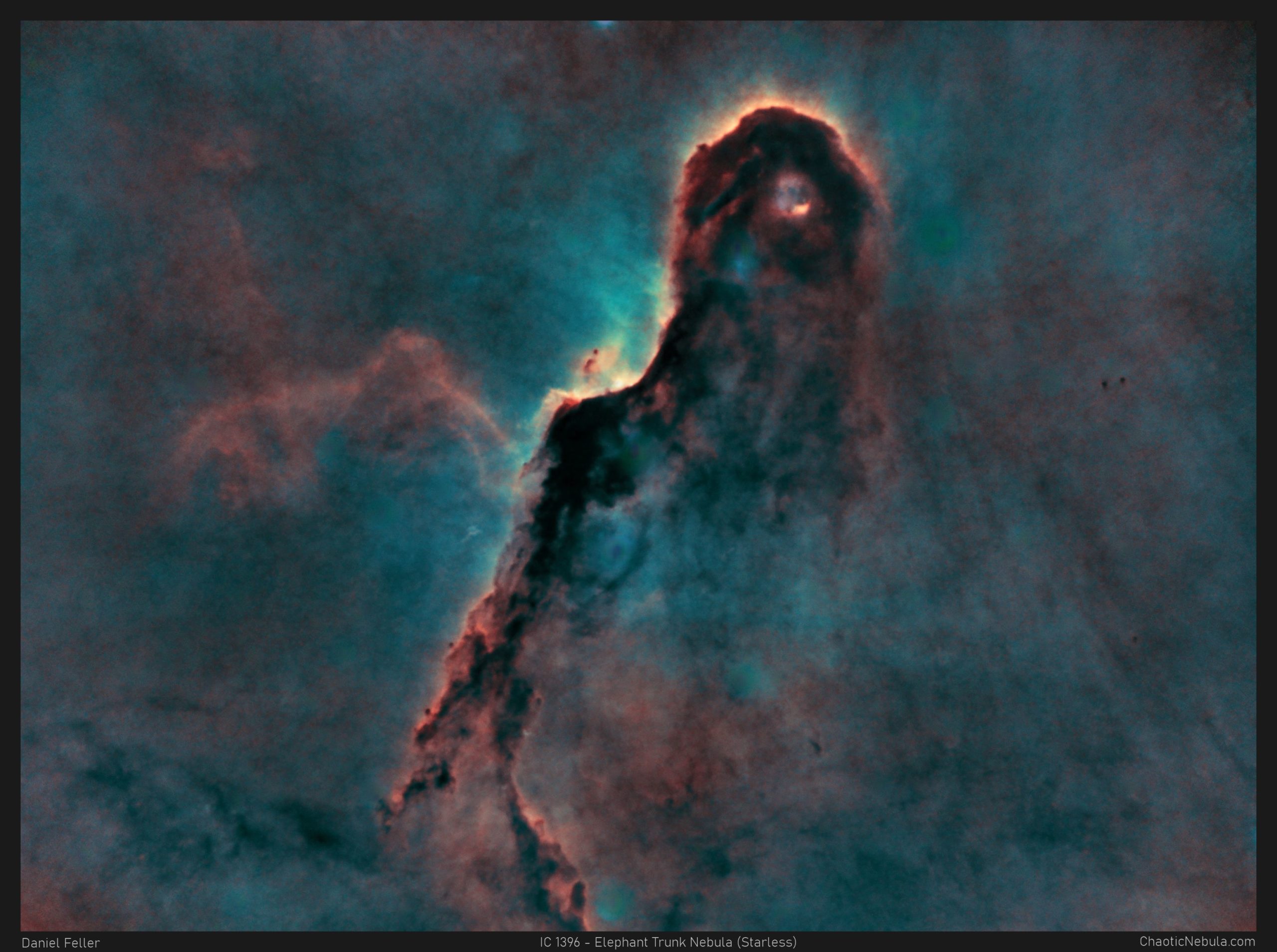
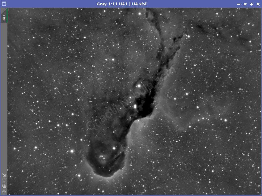
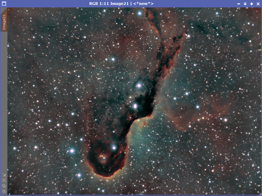
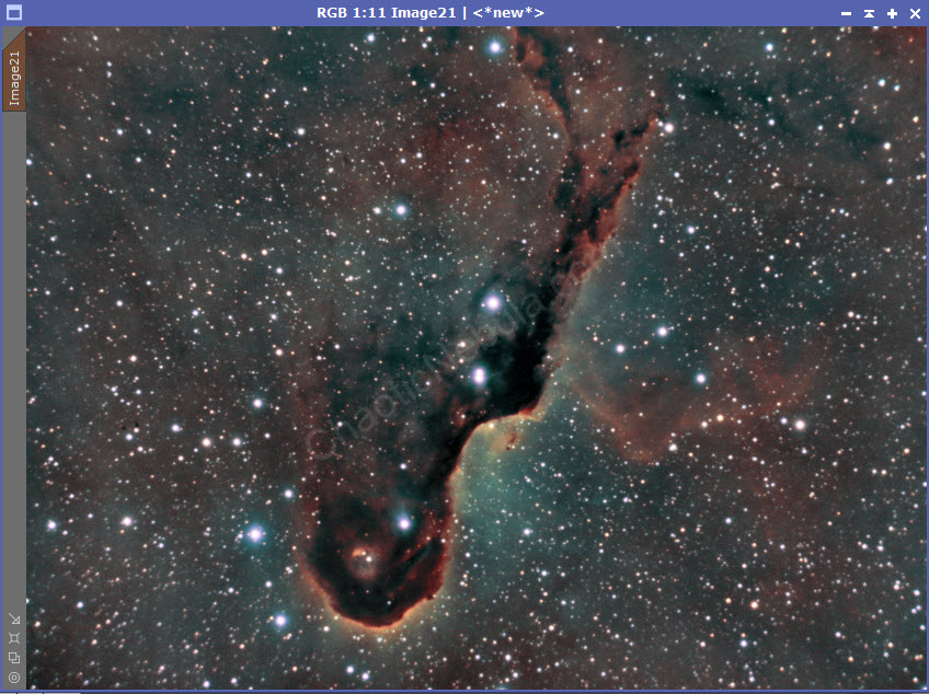
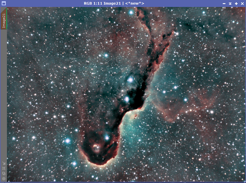
Can you spot the Elephant’s Trunk in the image?

The large round and dark section at the top, is the elephant’s head. The hole represents the elephant’s eye. And the long, dark stream coming off of the head is the trunk.

The Elephant Trunk Nebula (IC 1396A) is part of a much larger nebula, identified as IC 1396. The entire nebula spans over 100 light years and is located 2,400 light years away in the constellation Cepheus, while the trunk portion spans roughly 20 light years.

The Elephant Trunk Nebula is a is a concentration of gas/dust within a much larger emission nebula. The trunk is a recently discovered, active star forming region containing over 250 young stars (around 100,000 years old).

Imaging Details

Processing Workflow: Narrowband
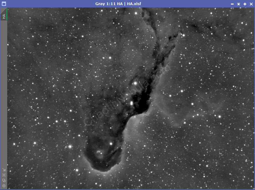
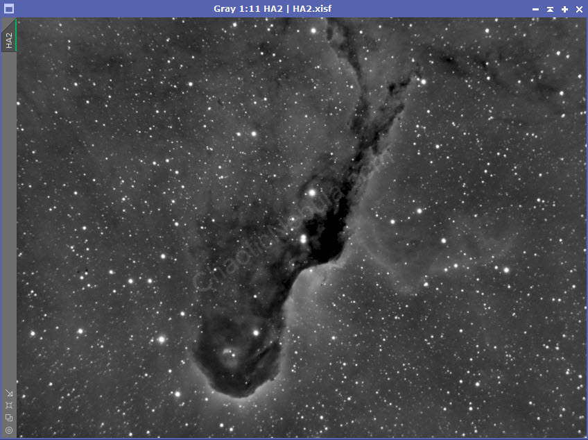
HA: 60*600 seconds
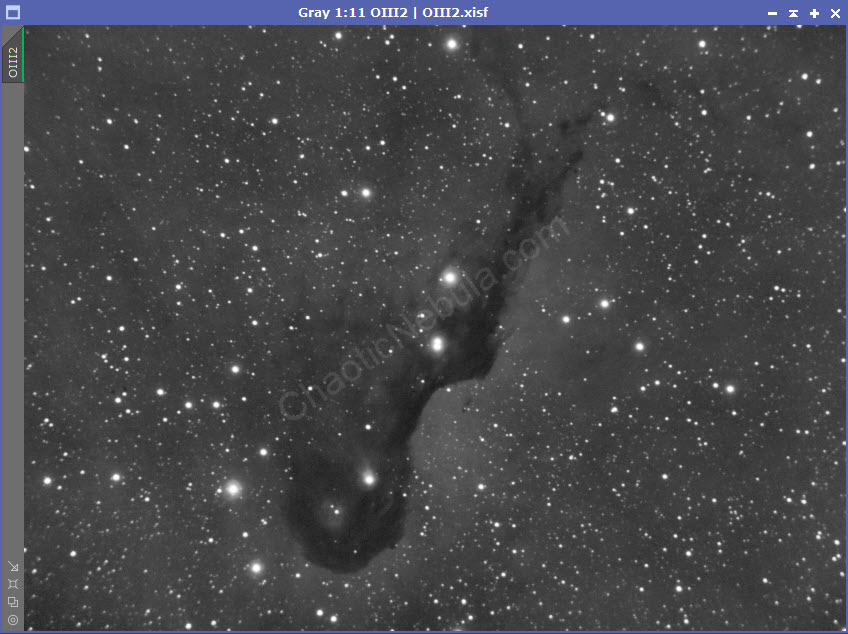
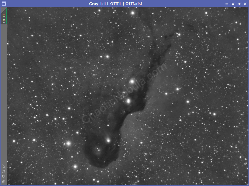
OIII: 120*600 seconds
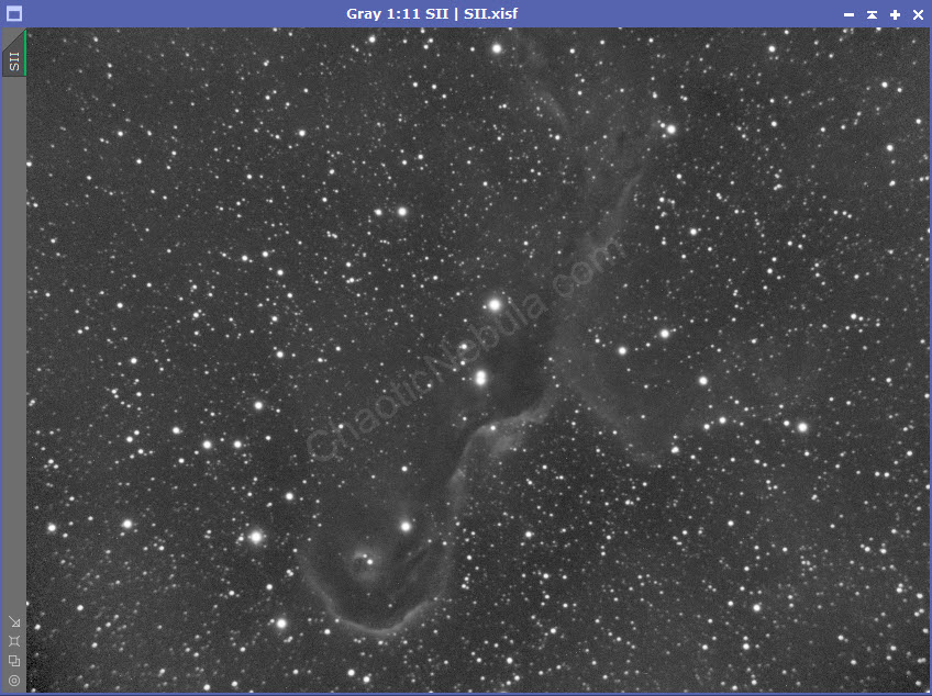
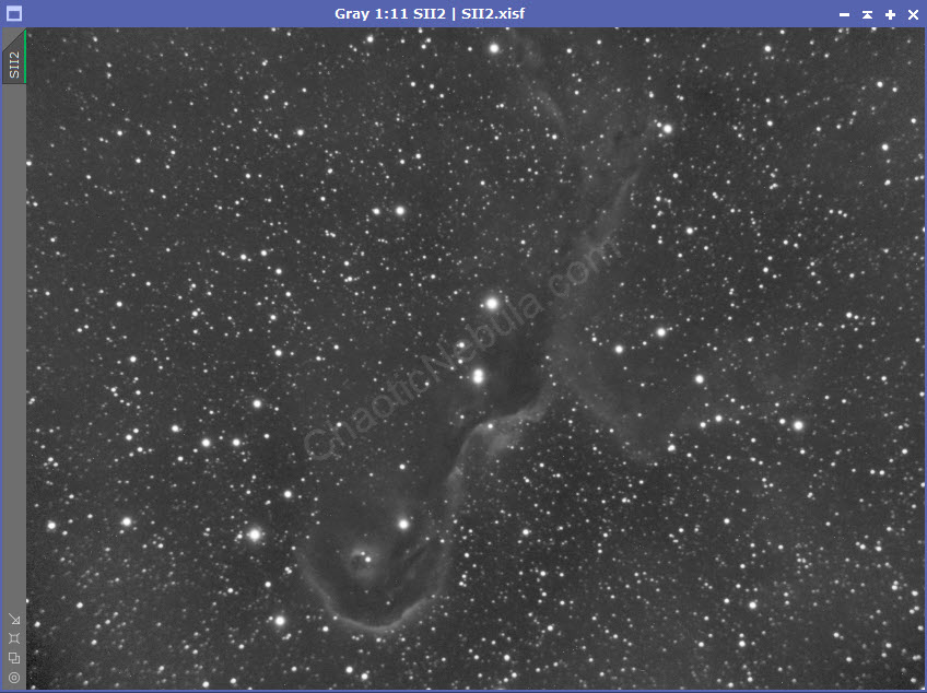
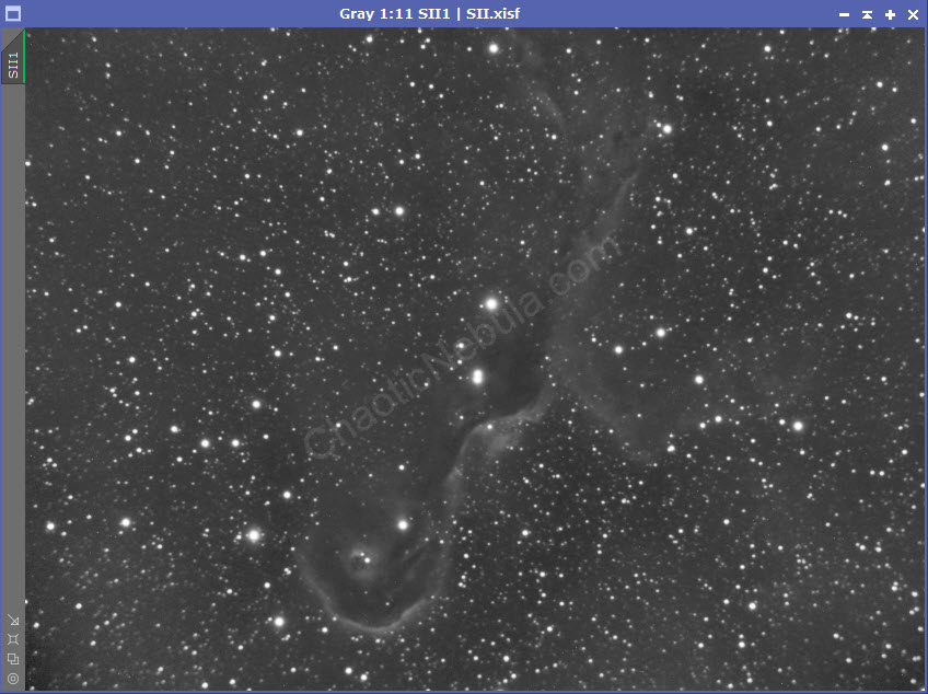
SII: 60*600 seconds
Total Imaging Time: 40 hours
Imaging Dates (8 nights):
- 8/3/2022
- 8/9/2022
- 8/20/2022
- 8/21/2022
- 8/30/2022
- 8/31/2022
- 9/3/2022
- 9/4/2022

Imaging Notes

My processing routine was based off of my Narrowband workflow. However, I did modify the process flow, which I will explain further when I have more time. A few additional items

Number of Images: I initially had 10 hours of OIII data, but as I kept having clear skies, and the nebula was positioned nicely in the sky, I decided to try and capture more. This resulted in 20 hours of OIII data. Although my signal-to-noise ratio improved slightly, it didn’t make a big impact. I will most likely continue capturing 10 hours of data per filter moving forward.
Starless Image: I used Starnet within PixInsight to generate the starless image. This was done at the very end of the processing routine.
Star Brightness: I often use Morphological Transformation to reduce the brightness of the stars and let the nebula shine through. After comparing the two images, I felt that the unmodified stars made the entire image brighter and more impressive. Dimming the stars made the image rather dull. Plus, the starless image helps show the detail with the dust lanes.

Imaging Workflow

My workflow changed slightly for this image. And based on the results, I might end up making this my preferred approach, although I plan to try this out on a few more images before changing my official narrowband workflow.

Integrated Image

I started off with three really good images for HA, OIII, and SII. I did my normal integration process with drizzle integration, dynamic crop, and dynamic background extraction.

OIII - Initial Image — HA – Initial Image

Noise Reduction

I followed my normal noise reduction process, first starting with TGV Denoise. I ran this process twice

The second part of noise reduction was to use multi-scale linear transformation.

Luminance Extraction

Before I stretched the image, I wanted to extract luminance. To achieve this, I did a linear fit, using the OIII image as the reference. I applied this to my HA and SII images.

I used channel combination to merge the three channels into an RGB image, with SII=Red, HA=Green, and OIII=Blue.

At this point, I’m not worried with how the colors appear. I simply need all channels combined together, so I can get a full luminance image. To achieve this, I simply use channel extraction to generate the luminance channel.

I’ll save this file for later.

Channel Combination

This is the point where my process diverges. The HA image is overpowering, making it hard to see the details from the other two channels. If you compare the HA and OIII images, the locations where OIII has a strong signal, the HA also has a strong signal. HA will overpower the weaker OIII signal.

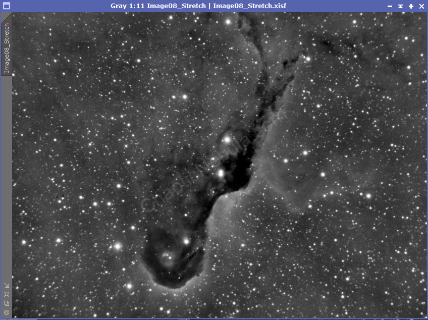
The new process first took my linear stretch images, and then did the same Histogram Transformation across all 3 images. This means all three images will receive the same stretch.

I used the following PixelMath formulas for this (credit to the thecoldestnights.com blog).

Red: (OIII^~OIII)*SII + ~(OIII^~OIII)*HA
Green: ((OIII*HA)^~(OIII*HA))*HA + ~((OIII*HA)^~(OIII*HA))*OIII
Blue: OIII

Color Saturation

With an integrated RGB image, I first increased the color saturation.

Luminance Integration

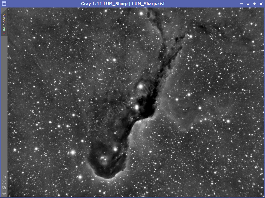
For the luminance image I saved earlier, I would normally run through my luminance workflow. However, deconvolution provided little value. I simply stretched and sharpened the image. As there aren’t extremely bright areas, I skipped HDR Transformation. And as for the Dark Structure Enhance, I also skipped as the dark structures in this image are already powerful.